Guide to Joint Fixity in Structural Modelling

How many times have you been up against a deadline and just idealized a connection as “pinned” or “fixed” to get the analysis to run? We’ve all been there. For decades, this simplification has been the bedrock of frame analysis, a necessary shortcut when we were armed with little more than slope-deflection and moment distribution. But in today’s world of performance-based design and powerful FEA software, clinging to this binary view isn’t just conservative—it can be inaccurate and uneconomical.

The reality is that most connections live in the grey area between these two extremes. They are semi-rigid, and their actual stiffness has a massive impact on everything from member sizes and frame stability to drift and seismic performance. For us in Canada, getting this right is critical for designing safe and efficient structures that comply with CSA S16 and the NBCC.

The Moment-Rotation (M-θ) Curve

Before we can analyze a semi-rigid connection, we need a way to describe its behaviour. That’s where the moment-rotation (M-θ) curve comes in. Think of it as the unique fingerprint of a connection. It plots the moment ($M$) the connection experiences against the relative rotation ($\theta$) between the beam and the column. This curve tells us everything we need to know about the connection’s performance.

Typical non-linear M–θ curve McGuire, Steel Structures, Prentice-Hall, 1968

A typical M-θ curve isn’t a straight line. Its shape reveals three key characteristics:

Initial Rotational Stiffness ($S_{j,ini}$): The slope of the initial, nearly-linear part of the curve. This tells you how stiff the connection is under service loads and is the main parameter for classification in CSA S16.
Moment Resistance ($M_{j,Rd}$): The peak moment the connection can handle before significant yielding. This is its ultimate strength.
Rotational Capacity (Ductility): The total rotation the connection can endure before losing its strength. This is critical for seismic design, where we rely on ductile connections to dissipate energy.

This rotation isn’t magic; it comes from real physical deformations like bolt elongation, plate bending, and shear deformation in the column’s panel zone. The M-θ curve neatly packages all that complex local behaviour into a single, usable relationship for our global frame analysis.

How to Classify Connections According to the Codes (CSA S16 & AISC)

Okay, so connections have unique M-θ curves. But how do we use that information in a standardized way? Both the Canadian and U.S. steel codes provide a harmonized system for classifying connections.

CSA S16-19 Stiffness Classification

The commentary to CSA S16 provides a clear, stiffness-based classification system. It uses a non-dimensional parameter, $K$, that compares the connection’s initial stiffness ($S_{j,ini}$) to the beam’s flexural stiffness ($EI_b/L_b$).

The formula is:

$$K = \frac{S_{j,ini} L_b}{E I_b}$$

Based on the value of $K$, CSA S16 defines three types of connections:

Simple (Pinned): If $K \le 2$. You may idealize the joint as transferring negligible moment.
Semi-Rigid (Partially Restrained - Type PR): If $2 < K < 20$. You must account for its stiffness and strength in your analysis.
Rigid (Fully Restrained - Type FR): If $K \ge 20$. The connection is stiff enough that it may be idealized as continuous for analysis (small end rotations still occur in reality).

For EITs: $L_b$ is the beam span, $E$ is Young’s modulus, and $I_b$ is the beam’s moment of inertia. This formula is essentially asking: “How stiff is the connection relative to the beam it’s attached to?” A very stiff connection on a very flexible beam will behave rigidly, and vice-versa.

Note: These $K$ limits are classification thresholds from commentary guidance intended to justify common idealizations. They are not statements that a joint is perfectly pinned or perfectly rigid; engineering judgement is still required.

AISC 360’s Two-Pronged System

It’s worth knowing the AISC 360 approach because it’s so prevalent in software and technical literature. The good news? The primary stiffness-based classification in the AISC 360 commentary is identical to the CSA S16 system, using the same formula and the same $K$ boundaries.

However, AISC also introduces a complementary strength-based classification, often called the “90%/20% rule.” This method looks at the connection’s moment strength relative to the plastic moment capacity of the connected beam ($M_p$):

Fully Restrained (FR): The connection can develop at least 90% of the beam’s plastic moment capacity. This ensures that if a plastic hinge forms, it will be in the beam, not the connection.
Partially Restrained (PR): The connection can develop between 20% and 90% of the beam’s plastic moment capacity.
Simple: The connection develops less than 20% of the beam’s plastic moment capacity.

Key Takeaway: Stiffness classification (CSA S16 & AISC) tells you how the frame will deform under service loads (governing drift and serviceability). Strength classification (AISC) tells you how the frame will fail at the ultimate limit state (governing failure mechanism and ductility). You need to consider both for a complete design.

From Graphical Methods to FEA

So, how do we actually incorporate this semi-rigid behaviour into our analysis?

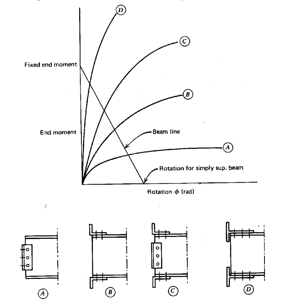
Classic Approach: The Beam Line Method

Before we had powerful software, engineers used a clever graphical technique called the beam line method. While you probably won’t use it for a final design today, it’s fantastic for understanding the underlying mechanics.

Here’s how it works:

Plot the Connection’s M-θ Curve: This is the “supply” curve—it shows how the connection can behave.
Plot the Beam Line: This is a straight line representing the “demand” from the beam and its loads. It’s derived from the slope-deflection equations. The line runs from the Fixed-End Moment (FEM) on the moment axis down to the free rotation (if it were pinned) on the rotation axis.
Find the Intersection: The point where the two lines cross is the equilibrium solution—the actual moment and rotation that will develop in that specific connection for that specific load.

Modern Approach: Rotational Springs in FEA

Today, our software does the beam line method for us numerically. We model the semi-rigid connection as a zero-length rotational spring at the beam-column joint.

The non-linear properties of this spring are defined directly by the connection’s M-θ curve. When you run a non-linear analysis, the software iteratively finds the equilibrium point for every single connection simultaneously, accounting for moment redistribution, P-Delta effects, and overall frame stability.

Pro-Tip: Don’t confuse Semi-Rigid Diaphragms with Semi-Rigid Connections. In software like ETABS or SAP2000, the “Semi-Rigid Diaphragm” option defines the in-plane stiffness of your floor slab for distributing lateral loads. It has nothing to do with the rotational fixity of your beam-to-column connections. They are completely separate inputs.

Modelling in Your Software

Applying this in your day-to-day work is more straightforward than you might think.

In S-FRAME: You can use the “Partial Release” feature. You specify a percentage from 0% (fully rigid) to 100% (fully pinned). This effectively applies a rotational spring at the joint proportional to the member stiffness (on the order of $EI/L$). This is great for early-stage design or sensitivity studies.
In SAP2000 / ETABS: You have more detailed options.
- Frame Hinges: You can define a non-linear hinge property by directly inputting the moment-rotation data from the M-θ curve and assigning it to the end of your beam element. This is essential for non-linear static (pushover) analysis.
- Link Elements: For the most control, you can use a zero-length “Link” element to connect the beam and column nodes. You then define the non-linear rotational properties of the link based on the M-θ curve. This is an extremely powerful method that can also model damping or gaps, making it ideal for advanced seismic devices.

Why This Matters for Engineers

This isn’t just an academic exercise. Accurately modeling joint fixity has huge implications for designing safe and economical buildings in Canada, especially when it comes to seismic design under NBCC and CSA S16, Clause 27.

More Economical Beams: By accounting for partial end restraint, you reduce the maximum positive moment at mid-span compared to a simple-span assumption. This often means you can use smaller, lighter, and cheaper beam sections.
Lower Seismic Forces (with caveats): A more flexible frame has a longer fundamental period ($T_a$). On the NBCC design spectrum, a longer period often means a lower spectral acceleration, $S(T_a)$, which can reduce the design base shear, $V$. Check NBCC minimum base shear provisions and SFRS limitations before relying on this reduction.
Ductile Behaviour and Capacity Design: Connections can be detailed to yield in a ductile manner so the frame dissipates energy while protecting primary members—this is the essence of capacity design in CSA S16 Clause 27. If you intend to claim higher ductility-related force modification factors ($R_d$), ensure your system conforms to a recognized SFRS category and its detailing requirements; unlisted systems should be treated conservatively.
Drift Control is Key: The trade-off for a more flexible, economical frame is increased lateral drift. A critical part of the design is rigorously checking your inter-storey drifts against the limits in NBCC to protect non-structural components.

In Practice vs. In Code: A fascinating Canadian case study of a modular steel school building found that standard welded stringer-to-beam connections, designed as pinned, actually exhibited significant semi-rigid behaviour. The finite element analysis showed a force redistribution that the simplified design model completely missed. It’s a stark reminder that even our “simple” connections often have inherent rigidity that we should be accounting for.

Your Next Steps

Moving beyond the pinned/fixed idealization isn’t just about refining your analysis—it’s about designing structures that more accurately reflect reality. It leads to more economical, efficient, and resilient buildings.

Here are three things you can do on your next project:

Question Your Assumptions: For a standard shear tab connection, do a quick check. Is it really “pinned”? Could the configuration be providing some rotational restraint that you could take advantage of?
Run a Sensitivity Study: In your model, try changing a few key connections from pinned (100% release) to partially restrained (e.g., 80% or 90% release in S-FRAME). See how it affects your beam sizes and frame drift. The results might surprise you.
Consult Connection Data: Look up M-θ data for common connection types. Resources from CISC, AISC, and research papers can provide the curves you need to model rotational springs accurately.

By embracing the reality of semi-rigid behaviour, we can move our designs forward, creating smarter and safer structures.

What’s the most common “simple” connection you’ve detailed that you suspect is actually providing significant rotational restraint? Share your thoughts in the comments below!

Disclaimer: This blog post is for informational purposes only and should not be taken as specific engineering advice. Always consult the latest edition of the National Building Code of Canada and relevant CSA standards for your projects.