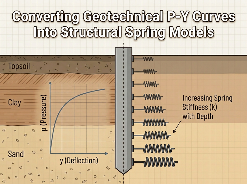
The geotechnical report lands on your desk with lateral pile capacity recommendations and a set of P-Y curves buried somewhere in the appendices. Your structural model wants spring values. How do you get from one to the other?
This translation problem sits on the boundary between two disciplines that don’t quite speak the same language. The geotechnical engineer works in soil mechanics and constitutive relationships. You work in springs and forces. Bridging that gap takes some effort, but the alternative is asking your colleague for “a spring constant” and getting numbers that may or may not match what your pile actually experiences.
Because soil doesn’t behave like a spring. The lateral pressure-displacement relationship is nonlinear, and any single stiffness value is a linearization at one specific displacement. To pick that displacement, you need analysis results. To run the analysis, you need a stiffness. That’s the loop you’re stuck with in soil-structure interaction.
What P-Y Curves Actually Represent
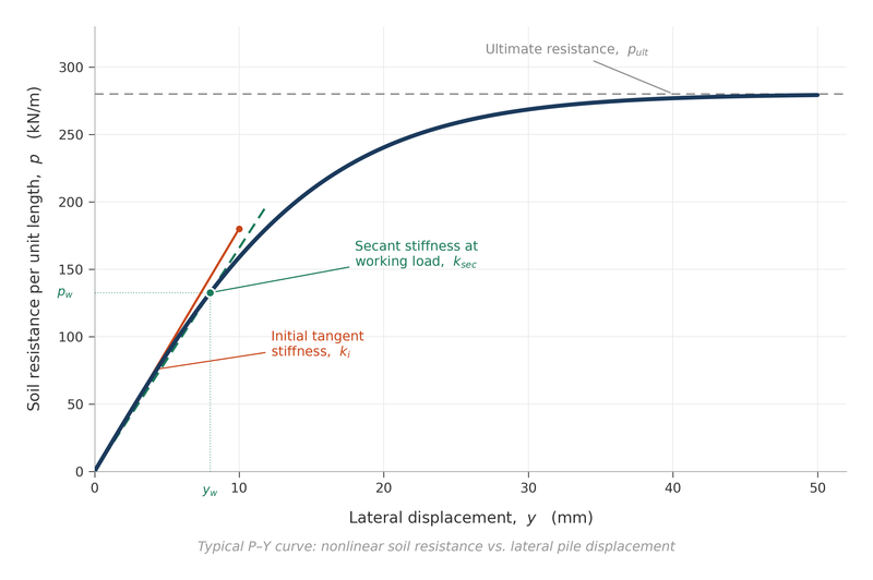
A P-Y curve is a force-displacement relationship for lateral soil-pile interaction at a specific depth. The “P” is lateral soil resistance per unit length of pile (typically in kN/m). The “Y” is lateral displacement (millimeters or meters).
Four behaviours show up in the curve shape:
- Initial stiffness: at small displacements, the response is stiff
- Progressive softening: tangent stiffness drops as displacement grows
- Ultimate resistance: the curve plateaus once soil reaches its limiting capacity
- Hysteresis: under cyclic loading, unloading and reloading paths diverge from the initial loading path (not shown on standard P-Y plots)
Curve shape depends on soil type, depth, pile diameter, and whether the loading is static or cyclic. Most geotechnical engineers generate these using API (American Petroleum Institute) correlations, which have been the industry default since the 1970s.
“API curves” refers to the P-Y formulations in API RP 2A, originally developed for offshore platform piles. They work for many onshore applications, but confirm applicability with your geotechnical consultant before relying on them.
The T-Z Curve: Axial Equivalent
P-Y curves cover lateral behaviour. T-Z curves cover axial load transfer along the pile shaft, where “T” is shaft friction per unit length and “Z” is axial displacement. The same nonlinearity rules apply: a pile mobilizes different amounts of shaft resistance at different settlement levels, and the T-Z curve tells you how that develops.
End-bearing piles also need a Q-Z curve for tip resistance versus tip displacement.
If your structural model has piles in it, you probably need P-Y, T-Z, and Q-Z data. Ask for all three when you coordinate.
Method 1: Secant Stiffness Approximation
The simplest way to convert a P-Y curve into a spring is the secant stiffness method:
- Estimate the lateral displacement your pile will see under design loads
- Draw a line from the origin to that point on the P-Y curve
- The slope of that line is your secant stiffness
where \(P_1\) and \(Y_1\) are the pressure and displacement at your expected load level.
The Iteration Problem
You need the displacement to pick the stiffness, but the stiffness sets the displacement. Three ways out:
Option A: Estimate and verify. Guess a displacement (10-25 mm covers most working loads), extract the secant stiffness, run the analysis, check if the result matches your guess. Iterate if not.
Option B: Multiple analyses. Run the model at several stiffness levels (say, 5, 10, 20, and 30 mm), then interpolate to find where input stiffness matches output displacement.
Option C: Conservative bound. Use the secant stiffness at maximum expected displacement. Lower stiffness, higher displacement, generally conservative for pile bending moments.
Iteration usually converges in 2-3 cycles. Wildly different displacements each pass mean the P-Y curve is steeply nonlinear in your operating range. Switch to piecewise linearization.
Converting to Discrete Springs
Once you have secant stiffness per unit length (kN/m per meter of displacement, or kN/m²), convert it to discrete spring values for your model.
For a pile discretized into segments of length \(\Delta z\):
$$K_{spring} = k_{secant} \times \Delta z$$If the geotechnical report gives you the coefficient of horizontal subgrade reaction (\(k_h\)) instead of P-Y curves, the spring stiffness is:
$$K_{spring} = k_h \times B \times \Delta z$$where \(B\) is the pile width or diameter.
Common Mistake: One spring stiffness for the whole pile length is wrong. Soil stiffness changes with depth, significantly for sands and less so for clays. Each spring needs the P-Y curve at its own depth.
Method 2: Piecewise Linearization
For pushover analysis, nonlinear time-history, or any case with significant displacement nonlinearity, secant stiffness loses too much. You need the curve shape.
Piecewise linearization approximates the nonlinear curve as connected linear segments:
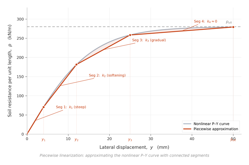
The process:
- Pick key points on the P-Y curve (initial slope, yield point, intermediate points, ultimate capacity)
- Connect them with straight segments
- Assign each segment a stiffness equal to its slope
- Use a multi-linear spring element in your analysis software
SAP2000, ETABS, and STAAD all support multi-linear spring definitions. Three to five segments captures the behaviour for most cases.
Practical Implementation
A typical breakdown for a medium-density sand P-Y curve:
| Segment | Y Range | Approximate k (normalized) |
|---|---|---|
| 1 | 0 to \(Y_1\) | 100% of initial |
| 2 | \(Y_1\) to \(Y_2\) | 40-60% of initial |
| 3 | \(Y_2\) to \(Y_3\) | 15-25% of initial |
| 4 | \(Y_3\) to \(Y_{ult}\) | ~0 (plateau) |
These numbers illustrate the pattern, not your actual curve. Use the values from your own P-Y data: stiff initial slope, progressive softening, plateau at ultimate capacity.
Depth Variation: The Part Most Models Get Wrong
Soil properties change with depth, so the P-Y relationship does too. This is the most oversimplified piece of lateral pile analysis I see in practice.
Sandy Soils
For sands, the coefficient of subgrade reaction usually increases linearly with depth:
$$k_h(z) = n_h \times z$$where \(n_h\) is a constant (kN/m³) and \(z\) is depth below ground. Deeper soil sits under higher confining pressure and behaves stiffer.
What that means for your model: the springs should get progressively stiffer down the pile. Near-surface springs are soft; deep springs are much stiffer.
Clayey Soils
Clays behave differently. Below roughly 6 pile diameters, the subgrade reaction is often near-constant with depth. The upper zone is where it varies, driven by:
- Reduced confinement near the surface
- Gap formation during cyclic loading
- Surface cracking in stiff clays
A good geotechnical report addresses this. If yours doesn’t, ask specifically about depth-dependent stiffness in the upper zone.
Practical Discretization
For typical piles:
- Closer spring spacing (0.5B to 1.0B) in the upper 5-10 diameters, where most bending occurs
- Wider spacing (1.0B to 2.0B) below that, where displacements are small
- Minimum of 8-10 springs along the active length
The active length, the depth over which significant lateral displacement occurs, runs 5-15 diameters for most pile-soil combinations. Below that the pile barely moves.
Coordinating With Your Geotechnical Engineer
Coordination starts with asking for the right things.
Request explicitly:
- P-Y curves at multiple depths (not just one)
- T-Z curve for shaft friction
- Q-Z curve for end bearing, if applicable
- Coefficient of subgrade reaction (\(k_h\)) and its depth variation
- Recommended soil damping for dynamic analysis
- Whether curves apply to static or cyclic loading (and if cyclic, the number of cycles assumed)
Provide to them:
- Pile diameter and stiffness (EI)
- Expected load levels (lateral force, moment at pile head)
- Loading type (static, cyclic, seismic)
- Expected displacement range, if you have a preliminary estimate
- Linear or nonlinear analysis
Pro Tip: A 30-minute call beats a week of email. Most misunderstandings come from the two disciplines using the same word for different things. “Stiffness,” “displacement,” and “spring” are the usual offenders.
The Language Gap
A translation table that helps:
| Structural Term | Geotechnical Equivalent |
|---|---|
| Spring constant | Secant stiffness from P-Y curve |
| Support reaction | Soil pressure × tributary area |
| Beam on elastic foundation | Pile with Winkler springs |
| Pushover analysis | Nonlinear static load-deflection |
| Modal period | Foundation flexible-base period |
When your colleague says “subgrade reaction,” they likely mean what you’d call “spring stiffness per unit length per unit width.” Same number, different framing.
Quality Control: Checking Your Springs
Before trusting your spring model, run a few sanity checks.
1. Order of magnitude check
For lateral stiffness of a single pile in medium-stiff soil:
- Initial spring stiffness: 10,000-50,000 kN/m (order of magnitude)
- Secant stiffness at 10 mm displacement: 3,000-20,000 kN/m
Values outside these ranges usually mean a unit conversion is off or an input is wrong.
2. Deflection profile check
Apply a simple lateral load case (say, 100 kN at pile head) and plot the deflection profile. It should peak at or near the head, decrease smoothly with depth, and approach zero within 10-15 diameters. Reversals, non-convergence, or excessive rotation point back to your spring assignments.
3. Moment diagram check
The maximum moment should land 2-5 diameters below ground for most single piles with lateral head loads. A maximum at a different depth, or discontinuities in the moment diagram, deserves investigation before you move on.
4. Comparison with hand methods
Cross-check against Broms’ charts or a beam-on-elastic-foundation solution. They won’t match exactly, but the result should be in the same ballpark. If it isn’t, find out why before you trust the detailed model.
A Worked Example: From P-Y Data to Model Springs
The geotechnical report gives you this P-Y curve for a 600 mm diameter pile in medium-dense sand at 3 m depth:
| Y (mm) | P (kN/m) |
|---|---|
| 0 | 0 |
| 5 | 120 |
| 10 | 180 |
| 20 | 240 |
| 40 | 280 |
| 80 | 300 |
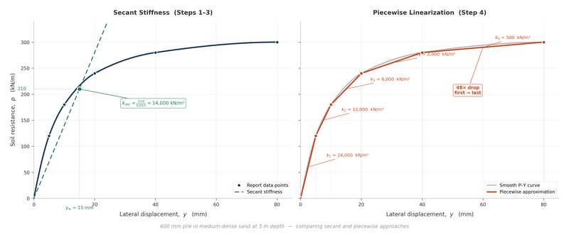
Step 1: Plot the curve and estimate expected displacement
Preliminary analysis points to about 15 mm displacement at this depth under design lateral loads.
Step 2: Calculate secant stiffness
Interpolating at \(Y = 15\) mm: \(P \approx 210\) kN/m
$$k_{secant} = \frac{210}{0.015} = 14{,}000 \text{ kN/m per m of pile}$$Step 3: Convert to discrete spring
With spring spacing \(\Delta z = 0.5\) m:
$$K_{spring} = 14{,}000 \times 0.5 = 7{,}000 \text{ kN/m}$$Step 4: For piecewise model (if needed)
Define segments:
- Segment 1: \(k_1 = 120/0.005 = 24{,}000\) kN/m² (0-5 mm)
- Segment 2: \(k_2 = 60/0.005 = 12{,}000\) kN/m² (5-10 mm)
- Segment 3: \(k_3 = 60/0.010 = 6{,}000\) kN/m² (10-20 mm)
- Segment 4: \(k_4 = 40/0.020 = 2{,}000\) kN/m² (20-40 mm)
- Segment 5: \(k_5 = 20/0.040 = 500\) kN/m² (40-80 mm)
Stiffness drops by almost 50x between the first segment and the last. A single secant value averages all of that into one number, which is why nonlinear analysis needs the segmented form.
When to Use Which Method
| Situation | Recommended Approach |
|---|---|
| Preliminary design, working loads | Secant stiffness at expected displacement |
| Final design, elastic range | Secant stiffness with iteration |
| Pushover analysis | Piecewise linear P-Y curves |
| Time-history analysis | Piecewise linear with unloading rules |
| Ultimate capacity check | Full nonlinear curve |
| Sensitivity study | Bound with high/low secant values |
For most routine projects in Canada, secant stiffness at 10-25 mm displacement is enough for pile foundation design. The full nonlinear treatment is worth the extra effort when you have:
- Large expected displacements
- Significant cyclic or seismic loading
- Performance-based design requirements
- Unusual soil conditions
Key Takeaways
Five things worth carrying forward:
Ask for curves, not constants. P-Y and T-Z curves carry the information you need. A single spring value bakes in assumptions you may not want.
Specify the displacement level. If you do need one number, tell your geotechnical engineer what displacement range you’re working at.
Respect depth variation. Soil stiffness changes with depth, particularly in the upper zone where most pile bending happens.
Iterate. The displacement-stiffness loop is circular by nature. Two or three passes resolve it.
Match complexity to purpose. Secant stiffness handles most projects. Nonlinear treatment is for projects that need it.
The gap between geotechnical and structural framing is real. What helps is spending enough time with the underlying soil mechanics that you can ask better questions in the first place.
References
- API RP 2A-WSD (2014). “Recommended Practice for Planning, Designing and Constructing Fixed Offshore Platforms,” American Petroleum Institute.
- Reese, L.C. and Van Impe, W.F. (2011). Single Piles and Pile Groups Under Lateral Loading, 2nd Ed., CRC Press.
- Bowles, J.E. (1996). Foundation Analysis and Design, 5th Ed., McGraw-Hill, Chapter 16.
- Das, B.M. (1999). Principles of Foundation Engineering, 4th Ed., PWS Publishing.
- FEMA P-751 (2012). “NEHRP Recommended Seismic Provisions: Design Examples,” Chapter 5.