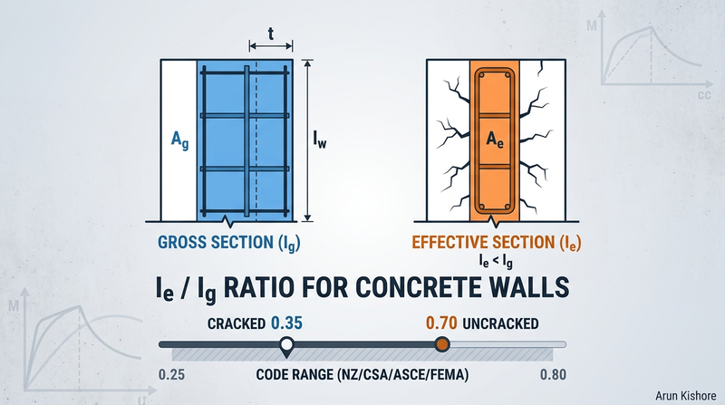
If you’ve ever looked up the effective moment of inertia ratio \(I_e/I_g\) for a concrete shear wall, you’ve probably noticed something frustrating: the values vary wildly depending on which code or guideline you consult, and critically, on what cracking state and loading condition they assume. The NZ Concrete Standard commentary suggests 0.25 for walls with no axial load. ASCE 41-23 recommends 0.35 for cracked walls. CSA A23.3 uses 0.7 for uncracked walls and 0.35 for cracked walls. FEMA 356 goes up to 0.8 for previously uncracked walls.
So which one is right? It depends.
Why can’t we just agree on a number?
The short answer: the effective stiffness of a cracked concrete wall isn’t constant. It changes based on several factors, and different codes have different target applications, cracking conditions, and hazard levels in mind.
When you model a concrete wall in your analysis software, you need to input an \(EI\) value. But concrete doesn’t behave linearly. It cracks, the reinforcement yields, and the stiffness degrades as you push further into the inelastic range. A single \(EI\) value is, at best, a reasonable approximation for a specific load level and performance objective.
Here’s what different guidelines recommend:
| Source | Condition | \(I_e/I_g\) Ratio |
|---|---|---|
| NZS 3101 Commentary (1995) | No axial load | 0.25 |
| NZS 3101 Commentary (1995) | With axial compression | 0.35 |
| ASCE 41-17/23 (Table 10-5) | Cracked walls | 0.35 |
| CSA A23.3 (Table 10.14.1.2) | Cracked walls | 0.35 |
| CSA A23.3 (Table 10.14.1.2) | Uncracked walls | 0.70 |
| FEMA 356 | Previously cracked walls | 0.50 |
| FEMA 356 | Previously uncracked walls | 0.80 |
Note that these values are not directly comparable. They correspond to different cracking states, axial load assumptions, and target performance levels. Comparing the NZ value for zero axial load (0.25) with the FEMA 356 uncracked value (0.8) as a “factor of three range” is misleading without this context. When you compare like-for-like conditions, the spread narrows considerably.
If you’re calculating periods, drifts, or force distributions, the choice still matters — but the right approach is to pick the value that matches your wall’s actual condition and your analysis purpose, not to pick the lowest or highest number from the table.
The moment-curvature reality
To understand where these numbers come from, think about the actual moment-curvature behaviour of a concrete wall section.
Before cracking, the wall responds with its gross section stiffness (\(EI_g\)). Once the concrete cracks, the stiffness drops, sometimes significantly. Push further and you’ll see reinforcement yielding, cover spalling, and eventually a plateau or degradation in capacity.
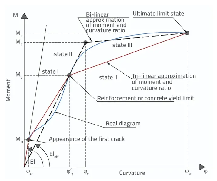 Typical layout of \(M-\phi\) diagram. Source.
The effective moment of inertia concept tries to capture this behaviour with a single value. The typical approach is to draw a secant line from the origin to some target point on the moment-curvature curve, usually the ultimate capacity at a curvature corresponding to your design drift limit.
Where you draw that secant line determines your effective \(EI\).
If your target performance is serviceability (limited cracking, essentially elastic response), you draw the secant to a point early on the curve, giving you a higher effective stiffness, maybe 0.7 or 0.8 of gross.
If you’re designing for life safety under a major earthquake and expect significant inelastic deformation, you draw the secant further along the curve, resulting in a lower effective stiffness, perhaps 0.25 to 0.5 of gross.
The “correct” \(I_e/I_g\) ratio depends on the performance level you’re targeting. There is no single right answer for all situations.
The axial load effect
One factor that significantly influences effective stiffness is axial compression. This often gets overlooked when engineers grab a single \(I_e/I_g\) value from the code without thinking twice.
Higher axial compression delays cracking. It pre-compresses the concrete, meaning you need more tension from bending before cracks form. The result is a stiffer response up to higher load levels.
This is explicitly acknowledged in the NZ Standard commentary, which recommends different values depending on whether the wall carries axial load: 0.25 for walls with no axial force and 0.35 for walls with axial compression. Research shows that walls with different axial load ratios (\(\frac{P}{A_g \cdot f'_c}\)) exhibit markedly different moment-curvature responses:
- At 5% axial load ratio: lower stiffness, earlier cracking
- At 10% axial load ratio: moderate stiffness improvement
- At 15-20% axial load ratio: noticeably higher effective stiffness
This is one reason the CSA A23.3 uncracked value of \(0.7I_g\) can be reasonable for many mid-rise concrete buildings, which often have moderate axial loads on their walls and may not experience significant flexural cracking under service or moderate seismic loads. But if you’re analyzing a slender wall in a low-rise building with minimal axial load that is expected to crack under design loading, 0.7 is unconservative for predicting drifts — and you should be using the cracked value of \(0.35I_g\) or performing a more detailed analysis.
If your wall has unusually high or low axial load, don’t blindly apply a single factor. Consider whether your situation warrants adjustment, and whether the wall will be cracked or uncracked under the relevant load level.
Boundary reinforcement matters too
The amount of reinforcement at the wall boundaries (those heavily reinforced zones at the ends of the wall) also affects effective stiffness.
More boundary reinforcement means:
- Higher ultimate moment capacity
- A different slope for the secant line to ultimate
- Generally higher effective \(EI\) for a given target curvature
Walls with minimum boundary reinforcement will show more stiffness degradation as they approach capacity compared to walls with generous boundary steel.
This is part of why performance-based seismic design guidelines often provide different stiffness modifiers depending on expected ductility demand. A wall expected to remain essentially elastic can use a higher effective stiffness than one expected to undergo significant plastic hinging.
What does CSA A23.3 actually say?
CSA A23.3, in Clause 10.14.1.2 (Table 10.14.1.2), specifies reduced stiffness values for concrete members used in elastic analysis with factored loads. For walls specifically, the code provides two values:
- Uncracked walls: \(0.7I_g\)
- Cracked walls: \(0.35I_g\)
The distinction depends on whether the wall is expected to crack under the applied loading, typically assessed by comparing the factored moment against the cracking moment based on the modulus of rupture.
What often gets missed: these values are intended for a specific context — force-based analysis where you’re looking at member forces under factored loads. They are not necessarily appropriate for:
- Drift calculations at serviceability limit states (where gross section properties are typically used)
- Period calculations for dynamic analysis
- Nonlinear analysis where you’re tracking stiffness degradation explicitly
For period calculations using elastic analysis, \(0.7I_g\) (uncracked) will give you a shorter period than the cracked value of \(0.35I_g\) would. To understand whether this is conservative, you need to think about where your building sits on the design spectrum. On the constant acceleration plateau, a shorter period gives you the same spectral acceleration — no penalty, but no benefit either. On the descending branch of the spectrum — where most mid- to high-rise wall buildings sit — a shorter period moves you up the curve to a higher spectral acceleration and therefore a higher base shear. This means that assuming uncracked stiffness when the wall is actually cracked is generally conservative for force calculations: you’ll overestimate forces. However, for drift predictions, using the uncracked stiffness when the wall is actually cracked will underestimate drift, which is unconservative.
When checking your analysis approach, ask yourself: “What am I using this stiffness for, and is my wall cracked or uncracked under this load level?” The answers should guide your choice of reduction factor.
A practical framework for choosing \(I_e/I_g\)
Rather than memorizing specific values, it helps to have a mental framework.
For force-controlled design (strength checks), higher \(I_e/I_g\) values (0.6-0.8) are often conservative because the resulting shorter period either keeps you on the constant acceleration plateau (same base shear) or moves you up the descending branch (higher base shear). Either way, you don’t underestimate forces. The CSA A23.3 uncracked value of 0.7 is reasonable for walls that aren’t expected to develop significant flexural cracking under the applied loads.
For drift-controlled design (deformation checks), lower \(I_e/I_g\) values (0.35-0.5) may be more appropriate. You want to capture the flexibility of the cracked system. Underestimating drift is unconservative. CSA’s cracked value of 0.35 — which aligns with ASCE 41’s cracked wall value — is a reasonable starting point.
For special situations: high axial load may justify increasing effective stiffness above the default cracked value. Slender walls with low axial load may need a decrease. Performance-based design should match stiffness to the target performance level — modern standards like ASCE 41-23 provide detailed guidance on this.
What you shouldn’t do:
- Ignore the cracked vs. uncracked distinction and always use 0.7
- Ignore axial load effects when they’re significant
- Apply residential building values to a high-rise core wall or vice versa
What requires judgment: running sensitivity analyses with different stiffness values and enveloping results can be a sound approach, but only when you understand which stiffness applies to which check and why. Mindless enveloping without understanding the underlying behaviour adds complexity without insight.
Why this matters for your projects
Getting the effective stiffness wrong has real consequences:
Force distribution: In buildings with mixed lateral systems (walls and frames), relative stiffness determines how forces split between elements. Overestimate wall stiffness and you might underdesign connecting frames.
Drift calculations: Underestimating flexibility means underestimating drift. You might miss a P-delta problem or undersize seismic joints.
Period and dynamic response: Your building period affects spectral acceleration, base shear, and expected response. It also affects torsional behaviour in irregular buildings.
Capacity design: If you’re doing capacity design for non-ductile elements, the stiffness assumption affects the demand you calculate.
A common mistake is using the same stiffness value for all analysis purposes without considering whether it’s appropriate for what you’re checking and whether your wall is cracked under the relevant load level.
Putting it into practice
Here’s a reasonable approach when starting a concrete building analysis:
Start with the code provisions. For CSA A23.3 applications, determine whether your walls are expected to be cracked or uncracked under the applied factored loads. Use \(0.7I_g\) for uncracked walls and \(0.35I_g\) for cracked walls per Table 10.14.1.2. This is a defensible starting point.
Check your axial loads. Are your walls carrying significantly more or less axial load than typical? Walls with high axial load ratios may remain uncracked at higher load levels, supporting the use of the higher stiffness value. Walls with low axial load will crack earlier.
Consider your analysis purpose. If you’re primarily checking forces, using higher stiffness (uncracked values) is generally conservative — it shortens the period and either maintains or increases base shear depending on where you sit on the spectrum. If you’re checking drifts, use the cracked stiffness or run a sensitivity check to understand the impact.
Document your assumptions. Whatever value you use, write down why. “Used \(0.7I_g\) per CSA A23.3 Table 10.14.1.2 for uncracked walls; wall axial load ratio approximately 10%; cracking check confirms wall remains uncracked under factored loads; primary concern is force distribution to frames” is much better than just “used \(0.7I_g\).”
Be consistent within each analysis. Don’t mix-and-match different stiffness assumptions for different walls without good reason (e.g., some walls genuinely cracked and others not).
Next steps
- Review your current project’s stiffness assumptions. Do they match the analysis purpose? Have you correctly assessed which walls are cracked vs. uncracked?
- Try running sensitivity analyses with \(I_e/I_g\) values at the high and low end of the typical range to see how your results change
- If you’re modelling walls as shell elements, make sure you’re also choosing the right element type for your analysis objectives
The range of code values for effective moment of inertia isn’t a sign of confusion in the profession. It’s a recognition that the “right” value depends on context — cracking state, axial load, performance objective, and analysis purpose. Understanding that context makes you a better engineer.
What stiffness assumptions are you using on your current project, and have you checked whether they match both your analysis purpose and your wall’s cracking state?