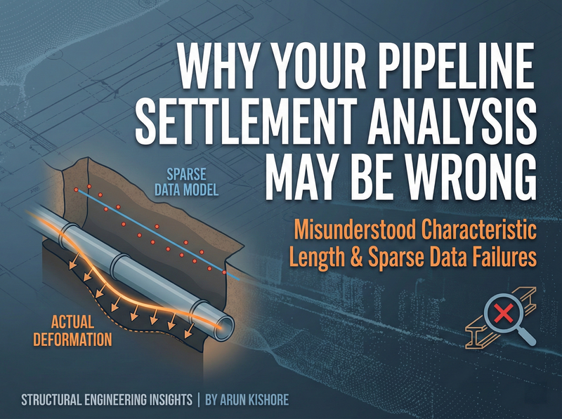
A buried 24-inch diameter pipeline running through a landfill on soft ground. Differential settlements measured at monitoring points spaced 15 to 25 metres apart. A dispute over who’s responsible for the damage. This case eventually made it to court, and the engineering analysis at the centre of it all contained fundamental errors that any engineer working on buried infrastructure needs to understand.
This post walks through the actual case, explains the theory behind the errors, and shows you how to think about these problems correctly.
The Setup: What Happened
A utility company had a pipeline running through a landfill on soft ground. A neighbouring property owner dumped material that caused significant ground settlement, and the pipeline was affected. Monitoring points were installed along the pipe, with survey stations typically spaced 15 to 25 metres apart. The measured settlements showed the pipe had moved, and the utility company took the matter to court seeking damages.
The engineer hired to analyze the pipeline did what seemed reasonable: build a beam model in a frame stiffness program, locate joints at the monitoring point locations, and impose the measured settlements as specified displacements at those joints.
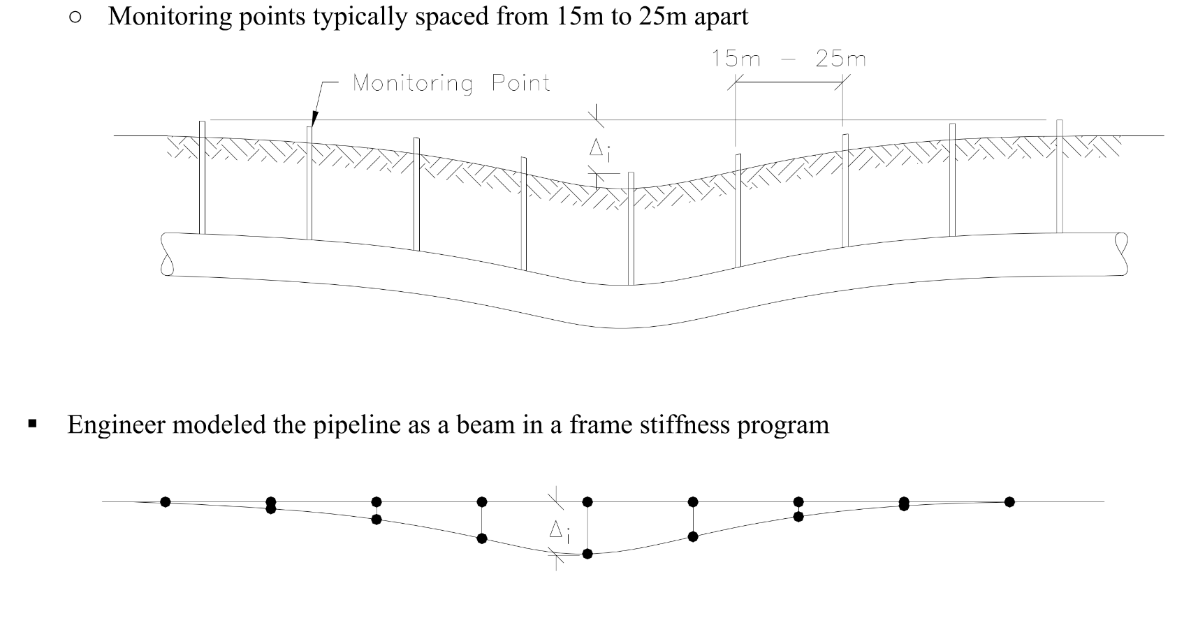
Source: SEABC Course C2 - Effective Modelling (2023)
The Core Problem: Characteristic Length
When you have a pipeline buried in soil, you’re not dealing with a simple beam. You’re dealing with a beam on elastic foundation - the pipe carries load, but the surrounding soil provides continuous support that resists deflection. This soil-structure interaction fundamentally changes how forces and moments distribute along the pipe.
For beam-on-elastic-foundation problems, there’s a key parameter called the characteristic length. For this particular pipeline, the characteristic length worked out to approximately 6 metres. The decay length - the distance over which effects from loading at one point die out - is about four times that, or roughly 24 metres.
Key Takeaway: The characteristic length tells you the scale at which your problem operates. Effects at one point propagate outward and essentially disappear within about one decay length.
What does this mean practically? If you want to get reasonably accurate stress results from discrete measurement points, those points need to be spaced no further apart than about half the characteristic length. For this pipeline, that’s approximately 3 metres.
The actual monitoring points? Spaced 15 to 25 metres apart.
The engineer’s input data was fundamentally too sparse to give reliable results, regardless of how sophisticated the analysis method. The structural theory tells us this before we even run the software.
Why Adding Nodes Didn’t Help
Here’s where the case gets instructive. When the uncertainty in the engineer’s results was pointed out, they attempted to validate the model by adding joints between the monitoring point locations. The thinking was that by refining the mesh, they could check for errors in the original analysis.
The result? Exactly the same stresses as before.
The engineer interpreted this as validation: “I refined my model and got the same answer, so the original must be correct.”
This interpretation reveals a fundamental misunderstanding of how frame stiffness methods work.
How Beam Elements Actually Behave
In a frame stiffness program, beam elements deform according to a cubic polynomial. This shape function exactly models situations where the bending moment varies linearly and shear is constant - which is precisely what happens between point loads.
When you impose displacements at specific nodes in a frame stiffness analysis, you’re essentially applying point loads at those locations. The beam elements between those points give you the exact solution for that loading condition. Not an approximate solution. The exact solution.
Pro-Tip: For point loads on beam elements, adding more nodes between load application points doesn’t improve accuracy. You already have the exact answer for that idealized problem.
So when the engineer added nodes between the monitoring points and got identical results, that wasn’t validation. That was the expected behaviour of the mathematics. The beam elements were already giving the exact solution for imposed point displacements (which is equivalent to point loads) at the original node locations.
Adding nodes between point loads is like measuring a straight line more times - you don’t get a more accurate answer, you just confirm what you already knew.
The Real Problem: Data Spacing vs. Reality
The engineer’s model gave exact results for the wrong problem.
The real pipeline experiences distributed loads from the settling soil, not point loads at discrete locations. The soil doesn’t suddenly push the pipe down at one spot and then do nothing for 15 metres before pushing down at the next spot. It applies pressure continuously along the pipe’s length.
To capture this distributed behaviour from discrete measurements, you need those measurements spaced closely enough to reconstruct the actual load distribution. Half the characteristic length is a practical minimum. The 15-25 metre spacing was roughly 3 to 4 times too coarse.
Frame Stiffness vs. Finite Difference: Bounds on the Answer
One way to understand the uncertainty is to compare different analysis methods on the same problem.
When you analyze the same pipeline with:
- Frame stiffness methods (point loads, exact cubic deformation between points)
- Finite difference methods (numerical approximation of the governing differential equation)
You typically find that frame stiffness results overestimate actual stresses while finite difference results underestimate them. The true answer lies somewhere between, but with widely-spaced data points, the gap between these bounds can be enormous.
In the actual case, the difference between methods was substantial - enough to make the stress results essentially meaningless for design or forensic purposes.
For Senior Engineers: When reviewing pipeline settlement analyses, always ask about the characteristic length of the soil-pipe system and compare it to the measurement spacing. If spacing exceeds half the characteristic length, the stress results should be viewed with skepticism regardless of how refined the computational mesh appears.
Two Problems, Not One
This case illustrates two distinct failures in understanding:
Problem 1: Not understanding the structural behaviour
The engineer didn’t recognize that beam-on-elastic-foundation problems have a characteristic length scale that governs how closely spaced your input data needs to be. This isn’t obscure theory - it’s fundamental to any buried infrastructure analysis.
Problem 2: Not understanding the numerical method
The engineer didn’t realize that frame stiffness methods already give exact solutions for point load problems. The “validation” exercise of adding intermediate nodes demonstrated ignorance of the underlying mathematics.
Both of these problems could have been avoided with a basic understanding of the theory before building the computer model.
What Should Have Been Done
If you find yourself in a similar situation - analyzing a pipeline with limited settlement data - here’s a better approach:
Calculate the characteristic length for your soil-pipe system. This depends on the pipe’s flexural stiffness and the soil’s modulus of subgrade reaction.
Compare your data spacing to the characteristic length. If your monitoring points are more than half a characteristic length apart, acknowledge that your stress results will have significant uncertainty.
Use appropriate analysis methods. If you must work with sparse data, consider methods designed for interpolation, or clearly bound your answer using multiple approaches.
Don’t validate by adding nodes between point load locations. You’re not testing anything meaningful.
Report the uncertainty honestly. In forensic or legal contexts, overstating confidence in results based on sparse data is both technically wrong and professionally dangerous.
For additional guidance on handling differential settlements with widely-spaced survey data, see Rajani and Zhan’s paper “Indirect estimates of flexural strain in concrete sidewalks induced by vertical movement” (Canadian Journal of Civil Engineering, Vol. 26, No. 3, June 1999, pp. 312-323).
Practical Takeaways
Before you run your next buried infrastructure analysis:
Know your characteristic length. For a beam on elastic foundation, it’s approximately \(L_c = \sqrt[4]{4EI/k}\), where \(EI\) is the beam’s flexural stiffness and \(k\) is the foundation modulus per unit length. The decay length is roughly \(4L_c\).
Check your input data density. Measurement points should be spaced at roughly half the characteristic length or closer for reliable stress results.
Understand what “exact” means. Frame stiffness beam elements give exact results for their assumed deformation shape (cubic polynomial). This is great for point loads, but it doesn’t mean your answer is exact for the real structure if the real loading is distributed.
Bound your uncertainty. Run multiple analysis methods if possible. When results diverge significantly, that tells you something important about data limitations.
Document your assumptions. Future reviewers (or opposing counsel) will want to know why you chose your analysis approach.
The engineer in this case likely ran sophisticated software and produced professional-looking output. But none of that matters if you don’t understand the fundamental behaviour of the system you’re analyzing. The software gives you exact answers to the problem you posed - it’s your job to make sure you’re posing the right problem.
Have you encountered similar issues with beam-on-elastic-foundation analyses? What characteristic length scales have you worked with, and how did they influence your modeling decisions?